Demo ERforResearch
R. Heyard
ERforResearch_vignette.RmdThe complex methodology of the ER is rather straightforward to use,
even without knowledge in building Bayesian hierarchical models. First,
for illustration, we will load a mock data set in R. The
function get_mock_data() does exactly that.
# Load the mock data
data <- get_mock_data()
The dataset comprises 3 different panels, with 5 voter and 15
proposals each. Every one of these voters gives a score to each of the
proposals. For the first illustrations, we will only use one panel
(p1).
data_panel1 <- data %>%
  filter(panel == "p1")
The aim of this package is to be able to rank the proposals in a certain call or panel. The most straightforward way to do this, is to use the average of the scores a proposal received from all the voters:
# First ranking based on simple means:
data_panel1 %>%
  group_by(proposal) %>%
  summarise(avg = mean(num_grade)) %>%
  arrange(-avg)
## # A tibble: 15 × 2
## proposal avg
## <chr> <dbl>
## 1 #1 5
## 2 #2 4.6
## 3 #3 4.6
## 4 #4 4.6
## 5 #5 4.4
## 6 #6 4.2
## 7 #7 4
## 8 #8 4
## 9 #9 3.8
## 10 #10 3.6
## 11 #11 3.4
## 12 #12 3.2
## 13 #13 2.8
## 14 #14 2.8
## 15 #15 2.6Let us assume, we had funding to accept five proposals in panel 1. In
this case, we would accept and fund the proposals #1-5, with average
scores ranging from 5 to 4.4. The methodology in the
ERforResearch package allows us to incorporate the
information on the voters behavior (are they more or less strict in
giving grades to proposals?). Additionally to that, the Bayesian
hierarchical models (BHM) can incorporate random variation in the
grading of the proposals, for example, due to conflict of interests or
other one proposal is not grades by every voter, (Note that here no
voter had a COI). This happens very regularly in the grant peer review
process. For this reason we will use a JAGS model via the
rjags package to build such a flexible model. The
ERforResearch package includes a function to call a default
JAGS BHM model:
?ERforResearch::get_default_jags_modelThen, we have the possibility to simply use that default model and
sample from it using the get_mcmc_samples() function.
# !Just for illustration purposes we set the rhat threshold a bit higher.
# Make sure to leave it at the default value of 1.01 once the package-
# functionalities are understood.

# Estimate theta's
mcmc_samples_object <-
  get_mcmc_samples(
    data = data_panel1, id_proposal = "proposal",
    id_assessor = "assessor",
    grade_variable = "num_grade",
    path_to_jags_model = NULL,
          # NULL means we use the default model
    seed = 6,
    rhat_threshold = 1.05,
    dont_bind = TRUE)
## [1] "Default model is used (check get_default_jags_model function!)."
## Calling 4 simulations using the parallel method...
## All chains have finished
## Simulation complete. Reading coda files...
## Coda files loaded successfully
## Note: Summary statistics were not produced as there are >50 monitored
## variables
## [To override this behaviour see ?add.summary and ?runjags.options]
## FALSEFinished running the simulation
## Calculating summary statistics...
## Calculating the Gelman-Rubin statistic for 108 variables....
## [1] "Extension JAGS samples number 1."
## Calling 4 simulations using the parallel method...
## All chains have finished
## Simulation complete. Reading coda files...
## Coda files loaded successfully
## Note: Summary statistics were not produced as there are >50 monitored
## variables
## [To override this behaviour see ?add.summary and ?runjags.options]
## FALSEFinished running the simulation
## Calculating summary statistics...
## Calculating the Gelman-Rubin statistic for 108 variables....
## Calculating summary statistics...
## Calculating the Gelman-Rubin statistic for 108 variables....
## Calculating summary statistics...
## Calculating the Gelman-Rubin statistic for 108 variables....
## Calculating summary statistics...
## Calculating the Gelman-Rubin statistic for 108 variables....
# It took the model .... to converge:
mcmc_samples_object$conv_status
## [1] "Converged (with threshold set to 1.05)"
c(mcmc_samples_object$n_adapt,
  mcmc_samples_object$n_burnin,
  mcmc_samples_object$n_iter)
## [1] 1000 4000 20000
# With the latter object we can do some convergence diagnostics,
bayesplot::mcmc_trace(mcmc_samples_object$samples$mcmc,
                      pars = paste0("proposal_intercept[", 1:15, "]"))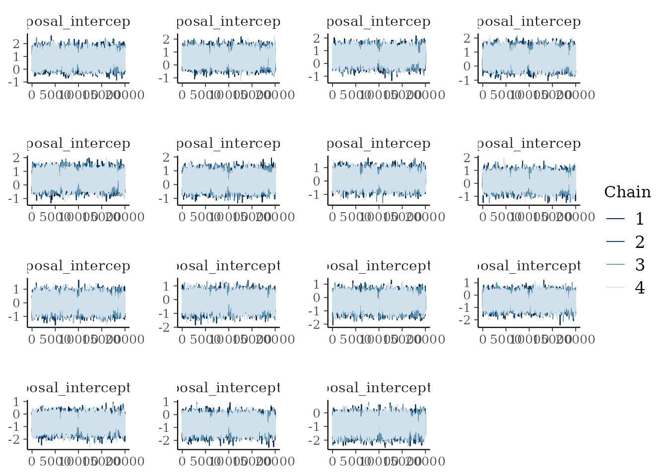
Traceplots of the proposal effects.
# Instead of the trace plots, we can directly look at the Summary in the object,
# which includes the rhat values (psrf), Monte-Carlo error (MCerr) and the
# effective sample size (SSeff) for each parameter, like so:
# mcmc_samples_object$summary

# If the model in path_to_jags_model is different from the default model with
# different names for the specific parameters, this has to be declared in the
# arguments (theta_name, tau_name, sigma_name, tau_voter_name, rank_theta_name).
# We can further produce rank histograms
pl1 <-
  bayesplot::mcmc_rank_hist(mcmc_samples_object$samples$mcmc,
                            pars = paste0("proposal_intercept[", 1:7, "]"))
pl2 <-
  bayesplot::mcmc_rank_hist(mcmc_samples_object$samples$mcmc,
                            pars = paste0("proposal_intercept[", 8:15, "]"))

pl1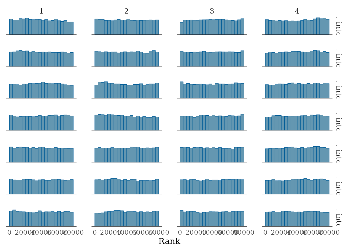
Rank histograms of the some parameters.
pl2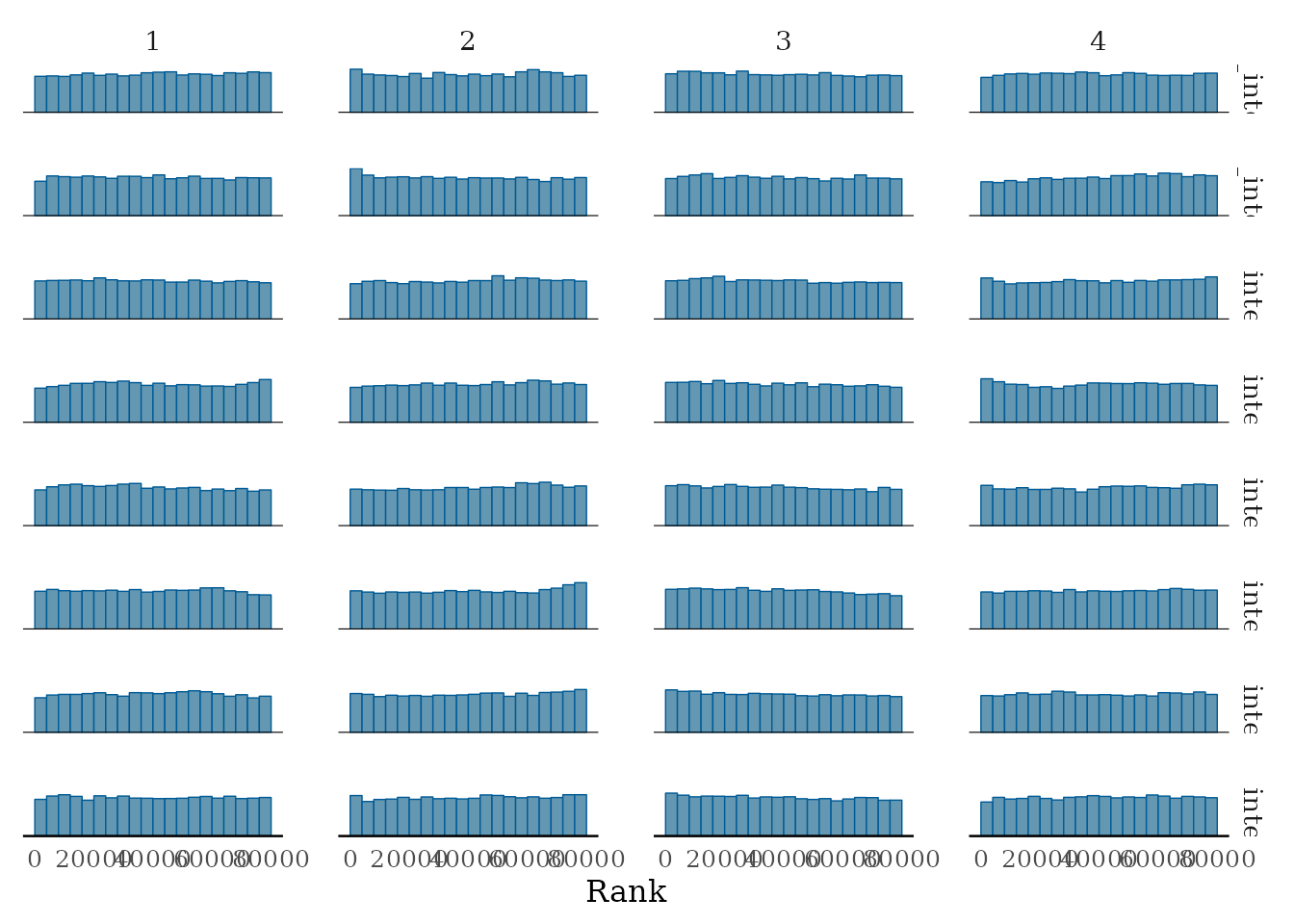
Rank histograms of the some parameters (continued).
# For the further analyis we will simply use all three chains
# and therefore bind them here.
mcmc_samples <- coda::mcmc(do.call(rbind, mcmc_samples_object$samples$mcmc))
We do not have to separately sample from the model, as the functions
that follow can easily call the get_mcmc_samples()
themselves. If the same seed is given to the seed argument
in the respective functions the results are reproducible.
Then, we use the plot_rankogram() function to plot the
Rankograms of each proposal, which are the probabilities of
each rank plotted against all possible ranks.
plot_rankogram(data = data_panel1,
               id_proposal = "proposal",
               id_assessor = "assessor",
               grade_variable = "num_grade",
               mcmc_samples = mcmc_samples_object
                  # if NULL the `get_mcmc_samples function is called from within
)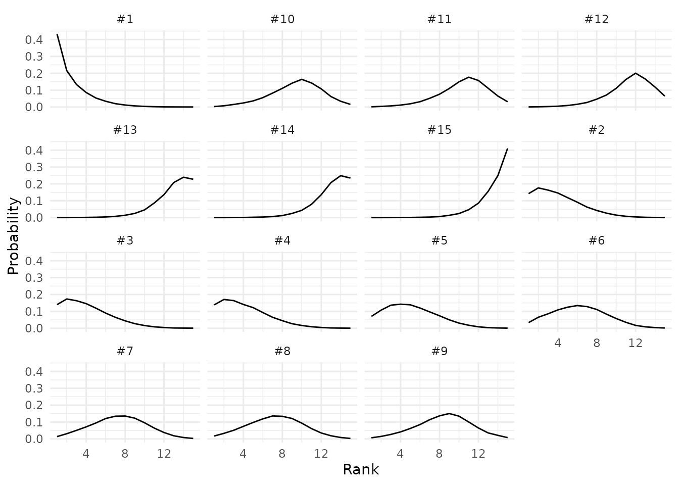
Rankogram for the proposals on the first panel.
Next, we can use the same function with the parameter
cumulative_rank_prob set to TRUE in order to plot the
cumulative ranking probabilities against the possible ranks.
plot_rankogram(data = data_panel1,
               id_proposal = "proposal",
               id_assessor = "assessor",
               grade_variable = "num_grade",
               cumulative_rank_prob = TRUE,
               mcmc_samples = mcmc_samples_object)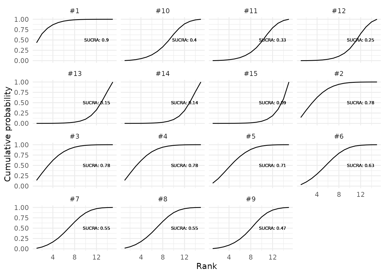
Cumulative ranking probability plots for competing proposals in the first panel.
The SUCRA is the area under the cumulative ranking probability plot. The higher the SUCRA value, the higher the likelihood of a proposal being in the top rank or one of the top ranks.
SUCRA_results <- get_sucra(data = data_panel1,
                           id_proposal = "proposal",
                           id_assessor = "assessor",
                           grade_variable = "num_grade",
                           mcmc_samples = mcmc_samples_object)
SUCRA_results$sucra %>% round(2)
## #1 #2 #3 #4 #5 #6 #7 #8 #9 #10 #11 #12 #13 #14 #15
## 0.90 0.78 0.78 0.78 0.71 0.63 0.55 0.55 0.47 0.40 0.33 0.25 0.15 0.14 0.09Finally we will compute the expected ranks (ER), which can directly be linked to the SUCRA. The lower the ER the better the evaluation of the proposal. The best possible ER is 1 for rank 1.
ER_results <- get_er_from_jags(data = data_panel1,
                               id_proposal = "proposal",
                               id_assessor = "assessor",
                               grade_variable = "num_grade",
                               mcmc_samples = mcmc_samples_object)

ER_results$rankings %>%
  mutate_if(is.numeric, function(x) round(x, 2)) %>%
  arrange(er)
## # A tibble: 15 × 6
## id_proposal rank avg_grade er rank_pm pcer
## <chr> <dbl> <dbl> <dbl> <dbl> <dbl>
## 1 #1 1 5 2.44 1 12.9
## 2 #2 3 4.6 4.06 2 23.7
## 3 #3 3 4.6 4.09 3 24.0
## 4 #4 3 4.6 4.12 4 24.2
## 5 #5 5 4.4 5.08 5 30.6
## 6 #6 6 4.2 6.19 6 37.9
## 7 #8 7.5 4 7.26 7 45.1
## 8 #7 7.5 4 7.34 8 45.6
## 9 #9 9 3.8 8.43 9 52.9
## 10 #10 10 3.6 9.42 10 59.4
## 11 #11 11 3.4 10.4 11 66.3
## 12 #12 12 3.2 11.4 12 73.0
## 13 #13 13.5 2.8 13.0 13 83.1
## 14 #14 13.5 2.8 13.0 14 83.6
## 15 #15 15 2.6 13.7 15 87.9The latter, can also be plotted using the
plotting_er_results function. As can be seen in the figure,
the five best proposals are still the same, but the ordering of all
proposals changed. The ER actually does a comparative ranking, by
comparing every proposal to every other proposal.
plotting_er_results(ER_results, title = "Panel 1", how_many_fundable = 5,
                    draw_funding_line = FALSE)
## Warning: attributes are not identical across measure variables;
## they will be dropped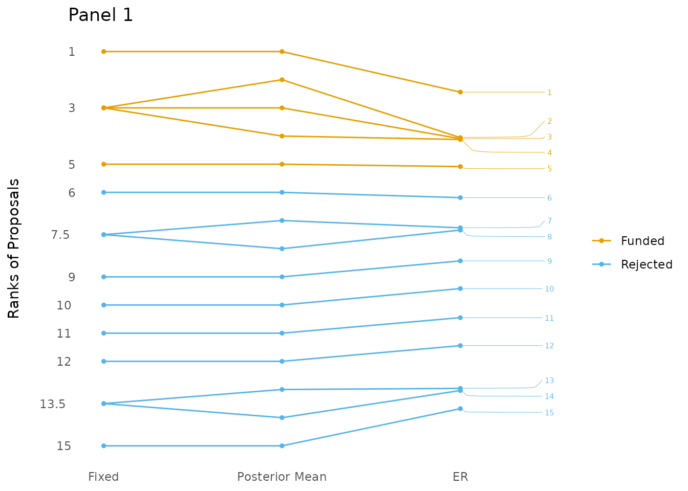
All proposals from the first mock panel ranked using the average grade (Fixed), the posterior means (Posterior Mean) and the expected rank (ER).
To better see, whether the funding line (FL) (here: between the fifth and the sixth proposal) goes through a cluster, we use the posterior distribution of the ER. The ERs of the competing proposals are plotted together with their 50% credible intervals (CrI). A provisional FL is defined at the ER of the last fundable (here the fifth) proposal. The proposals with a 50% CrI not crossing the FL are directly accecpted or rejected, depending whether their ER is lower or higher than the FL. The proposals with a 50% CrI crossing the FL will constitute the random selection group. In the case of panel 1 of the mock data four proposals will be randomly selected from a group of five.
plot_er_distributions(mcmc_samples_object,
                      n_proposals = data_panel1 %>%
                        summarise(n = n_distinct(proposal)) %>% pull(),
                      number_fundable = 5)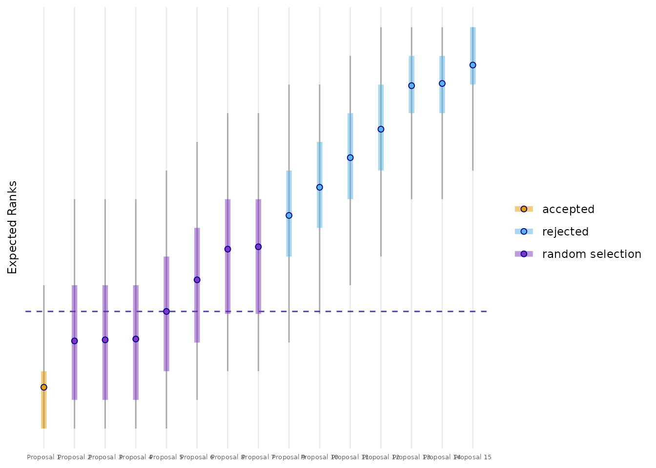
All proposals from the first mock panel ranked by their ER together with their 50% credible intervals (inner band) and 90% credible intervals (outer band).
The flexibility of the method of the ER allows us to not only look at
the panels individually but also rank all the proposals from the three
panels in one large ranking. To do this, we can simply use the default
model, but have to give a parameter for id_section.
## model{
##       # Likelihood:
##       for (i in 1:n) { # i is not the application but the review
##           grade[i] ~ dnorm(mu[i], inv_sigma2)
##                 # inv_sigma2 is precision (1 / variance)
##           mu[i] <- overall_mean + proposal_intercept[num_proposal[i]] +
##           assessor_intercept[num_assessor[i]] + panel_intercept[num_panel[i]]
##       }
##       # Ranks:
##       rank_theta[1:n_proposal] <- rank(-proposal_intercept[])
##       # Priors:
##       for (j in 1:n_proposal){
##         proposal_intercept[j] ~ dnorm(0, inv_tau_proposal2)
##       }
##       for (l in 1:n_assessors){
##         assessor_intercept[l] ~ dnorm(nu[l], inv_tau_assessor2)
##       }
##       for (l in 1:n_assessors){
##         nu[l] ~ dnorm(0, 100) # 1/(0.1^2) = 100
##       }
##       for (l in 1:n_panels){
##         panel_intercept[l] ~ dnorm(0, inv_tau_panel2)
##       }
##       sigma ~ dunif(0.000001, 2)
##       inv_sigma2 <- pow(sigma, -2)
##       inv_tau_proposal2 <- pow(tau_proposal, -2)
##       tau_proposal ~ dunif(0.000001, 2)
##       inv_tau_assessor2 <- pow(tau_assessor, -2)
##       tau_assessor ~ dunif(0.000001, 2)
##       inv_tau_panel2 <- pow(tau_panel, -2)
##       tau_panel ~ dunif(0.000001, 2)
##     }
Then we use the latter model to directly plot the ER:
ER_results_all <- get_er_from_jags(data = data,
                                   id_proposal = "proposal",
                                   id_assessor = "assessor",
                                   id_panel = "panel",
                                   grade_variable = "num_grade",
                                   tau_name_panel = "tau_panel",
                                   n_chains = 4, n_iter = 5000,
                                   n_burnin = 1000, n_adapt = 1000,
                                   rhat_threshold = 1.1)
## [1] "Default model is used (check get_default_jags_model function!)."
## Calling 4 simulations using the parallel method...
## All chains have finished
## Simulation complete. Reading coda files...
## Coda files loaded successfully
## Note: Summary statistics were not produced as there are >50 monitored
## variables
## [To override this behaviour see ?add.summary and ?runjags.options]
## FALSEFinished running the simulation
## Calculating summary statistics...
## Calculating the Gelman-Rubin statistic for 769 variables....
## [1] "Extension JAGS samples number 1."
## Calling 4 simulations using the parallel method...
## All chains have finished
## Simulation complete. Reading coda files...
## Coda files loaded successfully
## Note: Summary statistics were not produced as there are >50 monitored
## variables
## [To override this behaviour see ?add.summary and ?runjags.options]
## FALSEFinished running the simulation
## Calculating summary statistics...
## Calculating the Gelman-Rubin statistic for 769 variables....
## Calculating summary statistics...
## Calculating the Gelman-Rubin statistic for 769 variables....
## Calculating summary statistics...
## Calculating the Gelman-Rubin statistic for 769 variables....
## Calculating summary statistics...
## Calculating the Gelman-Rubin statistic for 769 variables....
plotting_er_results(ER_results_all, title = "All three panels",
                    draw_funding_line = FALSE,
                    how_many_fundable = 15)
## Warning: attributes are not identical across measure variables;
## they will be dropped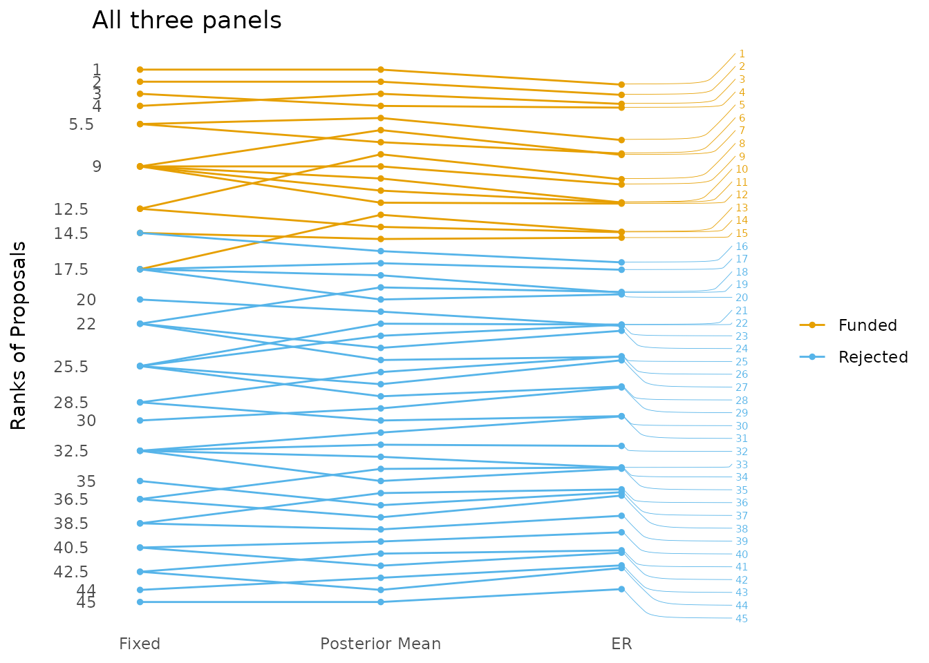
The proposals from all mock panels ranked using the average grade (Fixed), the posterior means (Posterior Mean) and the expected rank (ER).